Analytics as Code - Code, configs, and data version-controlled

Overview

Code is the only abstraction for managing complexity in software projects. From tools like Terraform that help you manage and provision your infrastructure as code (IaC), Kubernetes or Nomad for orchestrating containers, or to tools for managing policies or configs as code (CaC), defining your resources through code and version controlling them offers several advantages.

First of all, it guarantees consistency across executions. Applying a plan or a set of changes in different environments leads to the same output. Secondly, these tools are declarative. You define what your desired end state should be, and the tools manage all resource dependencies and know how to apply the changes to get to that state, even if sometimes it involves destroying and recreating resources in the process, without you having to define what steps it needs to take to get to that state. Thirdly, having all your configurations version controlled ensures an auditable process. Every change undergoes review, allowing code to be automatically linted and tested. Lastly, your setup is portable: you can export your latest infrastructure, configs, or other parts of the system to a different account or region only through a CLI command. These four aspects lead to a predictable and scalable system.

Applying the same concepts to the data world

So, how can we extend the benefits of code-based solutions to the analytics world? What would we need? Well, a couple of things:

All resources are created as code: Everything from data sources to models, to secrets and environment variables, orchestration groups, alerts, tests, and access control policies.
All resources are version controlled to ensure we have an auditable process that can be tested.
When making a change, automatic CI tests are executed, such as code linters (formatting), code coverage, stale assets, syntax errors (invalid model references {{ ref(‘inexistent_model’) }}).
When reviewing a pull request (PR), it should be clear what code and configurations have changed, which assets are updated, how the lineage is affected, and the data differences for the impacted assets.
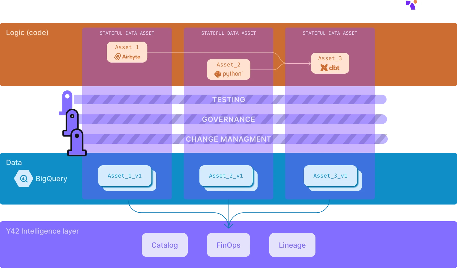
You declare the end state of your data assets, focusing on the desired outcome rather than managing resource dependencies or how assets are materialized in the data warehouse.
Linking code and configs to data. Each materialization of a data asset in the data warehouse is linked to a specific version of the code. This means that whenever you want to rollback to a previous version of your codebase or deploy a new version to production, the data warehouse is up to date to what you defined in code.

The last point is extremely important to achieve Analytics as Code. It’s not only code and configurations that needs to be version controlled, audited, and tested, but also data.

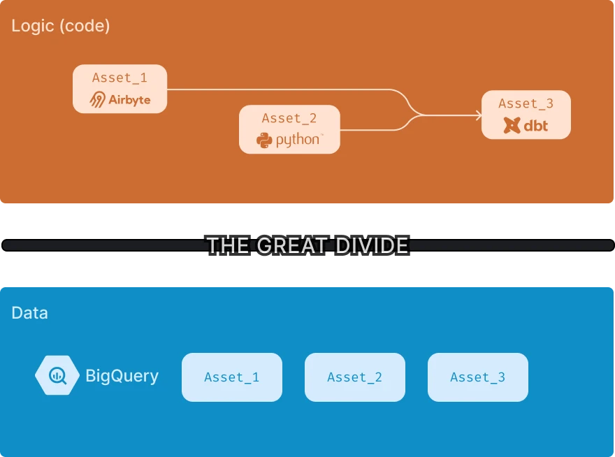
In a stateless system, the data and code don't know of each other.

In a stateless environment, the state of the codebase is decoupled from the state of the data warehouse. As organizations scale -- more models are created, more people are onboarded, or more assets are created -- the two worlds drift apart, and therefore, our intention that we declare through code may not be in sync anymore with the actual data in the data warehouse. For a deeper understanding of the importance of statefulness in data pipelines, you can read more in this blog post.

However, directly version controlling large-scale datasets is not possible yet – you can’t store terabytes of data in a repository, nor update it after every pipeline execution.

Versioning data in Y42: A new paradigm shift

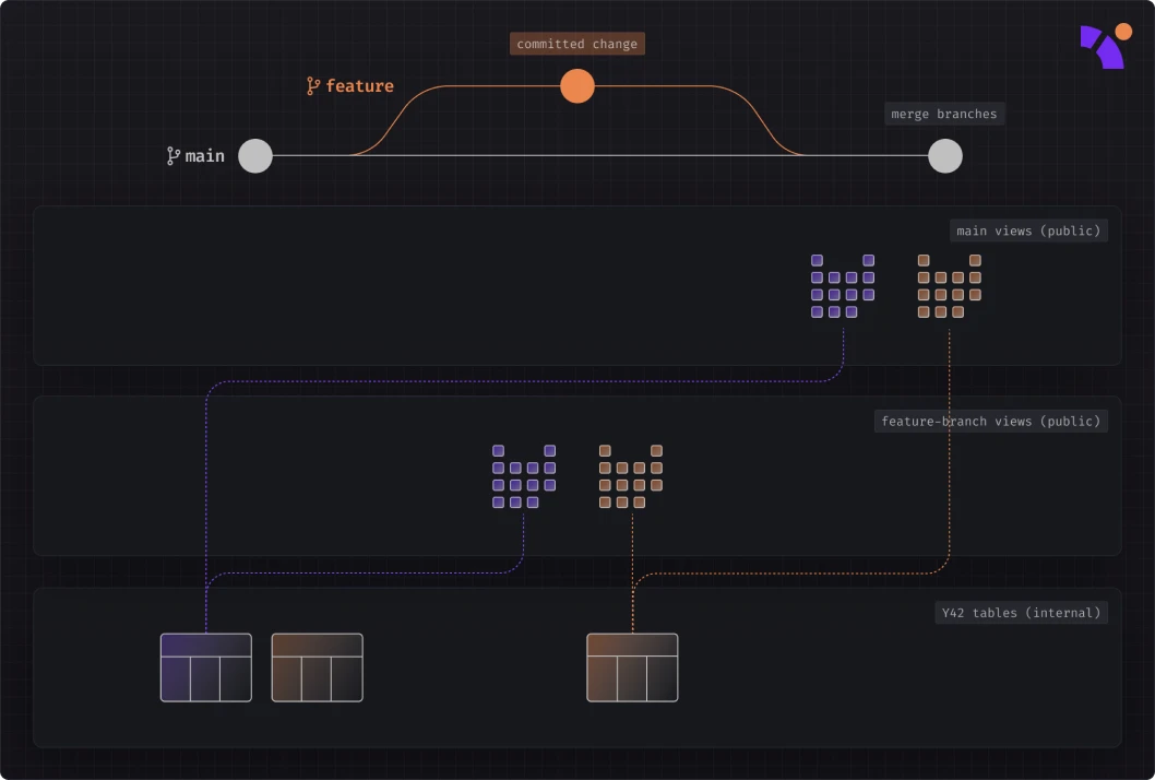
Our solution to data versioning involves building and maintaining links between the state of the codebase and the assets materialized in the data warehouse. To do this, we automatically create two schemas (or two datasets, depending on the database engine) in the data warehouse: a customer-facing schema with views and clones, and an internal schema managed by Y42. Any code change is first materialized in the internal schema, with a reference to it maintained in the customer-facing schema. When you create a feature branch or merge changes into the main branch, the customer-facing views and clones are automatically updated to point to the appropriate materialization in the internal schema. This approach not only ensures instant rollbacks and deployments but it’s also cost-effective, sometimes saving you up to 68% depending on the setup. You can read more about Virtual Data Builds and its benefits here.

Hands-on tutorial: Implementing analytics as code

In this article, we will look at some practical examples of what Analytics as Code means. We’ll begin by connecting two data sources: an Airbyte Postgres source, and a custom Python Ingest script. Next, we’ll create dbt models downstream by joining the two sources, and set up an orchestration group to run our pipeline every hour. We’ll then merge our changes into the production/main branch, and showcase how the Virtual Data Builds mechanism helps us reuse assets from our working environment/branch in production, so we don’t need to recompute our models.

Throughout the process, we’ll see how each UI action is backed by code and how the Y42 deep integration with git works. In the end, we will monitor the pipeline using Y42’s Asset Monitor dashboard.

In a follow-up article, instead of merging directly our code changes to production branch, we'll create a pull request (PR) and view the Y42 CI bot in action.

Let’s begin!

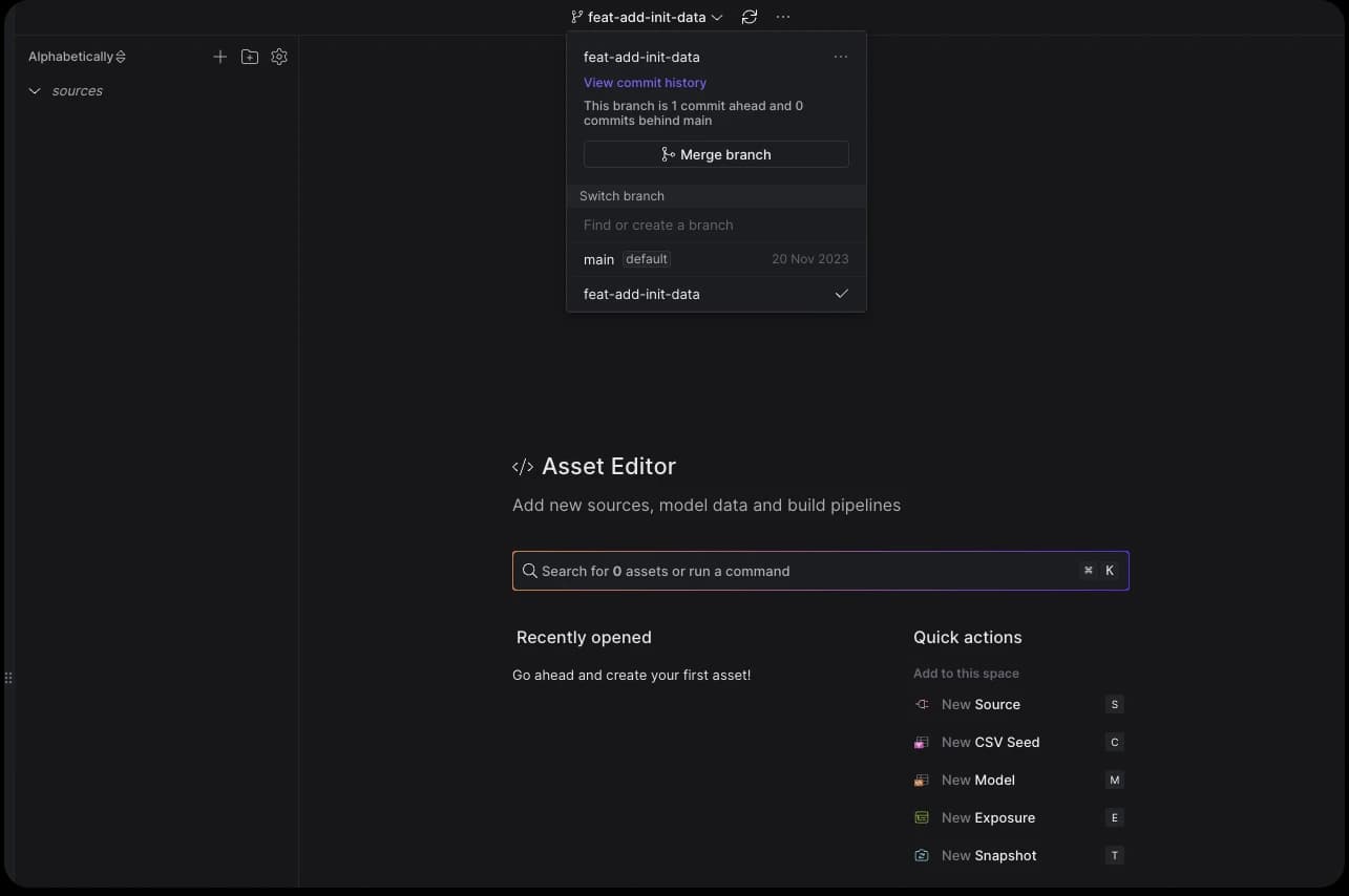
Creating a new feature branch

We’ll start by creating a new branch from the main branch.

Add an Airbyte Postgres source

First, we'll configure an Airbyte source to pull data from a Postgres database. This database contains the Pagila sample data, a Postgres adaptation of the MySQL-compatible Sakila sample database.

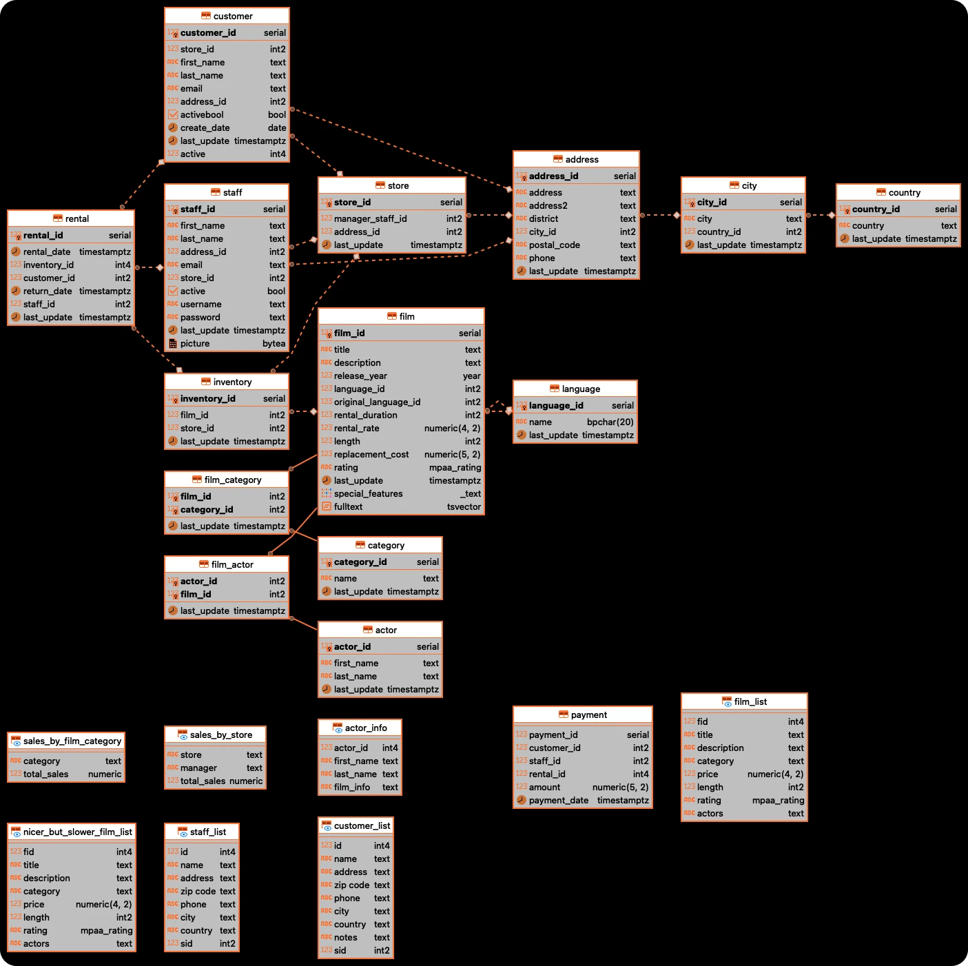
To follow along, you can replicate the input database using the instructions in Aiven’s documentation.

wget https://raw.githubusercontent.com/aiven/devportal/main/code/products/postgresql/pagila/pagila-data.sql
psql 'SERVICE_URI'
CREATE DATABASE pagila;
\c pagila;
\i pagila-data.sql;
\c pagila;

I've set up a Postgres database using Google Cloud SQL. To configure it, first head to the Networking tab. In the Authorized networks section, add the IP address (35.198.72.34). This step allows Y42 to initiate requests to your database.

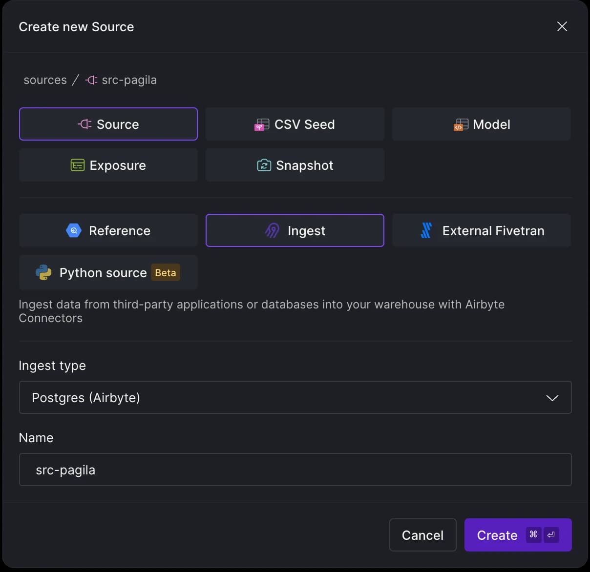
Once your source database is populated with data, switch to Y42. Press CMD + K and choose New Source. Select Ingest (Airbyte) and then choose Postgres as your Ingest (Source) type.

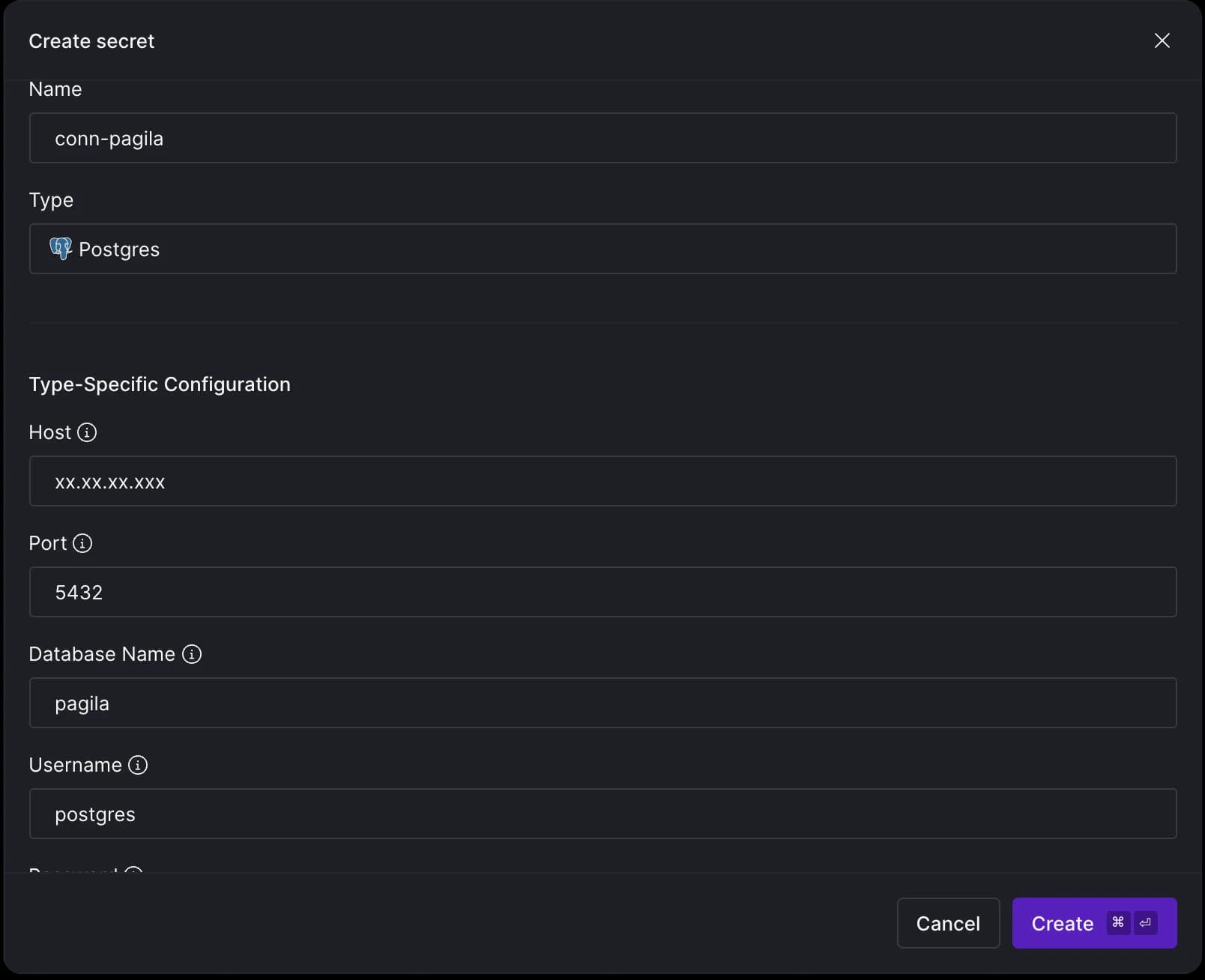
Now, we will be prompted to enter our credentials for the Postgres instance:

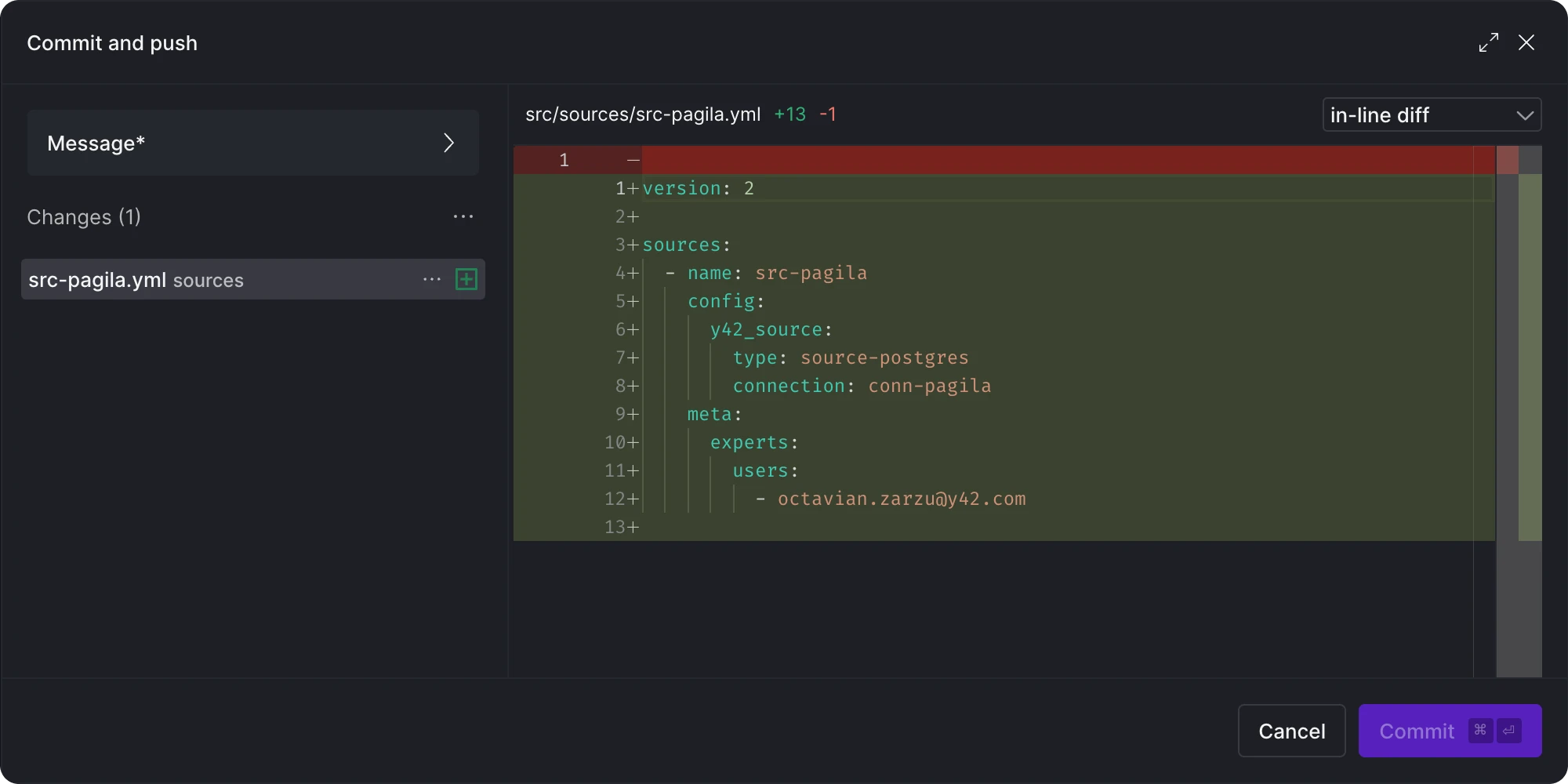
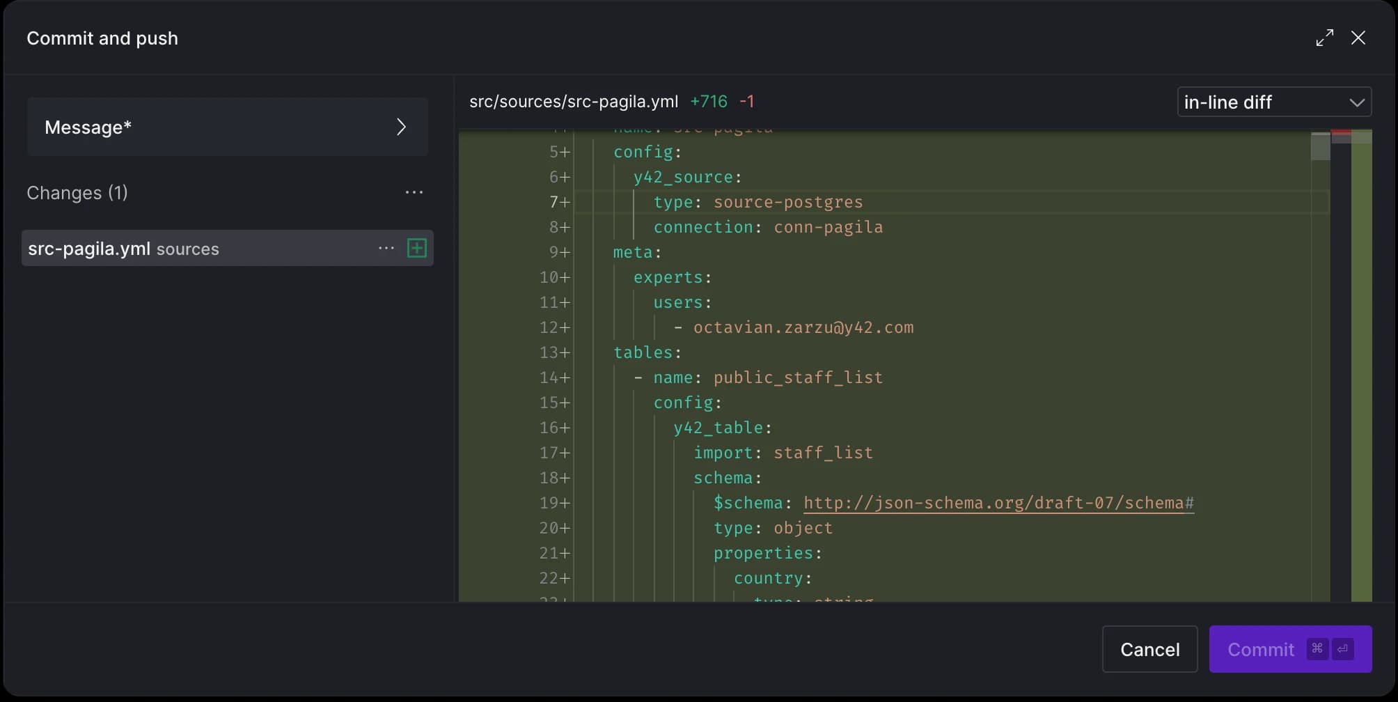
At this stage, you'll notice there is one file ready to be committed, which relates to the source we just set up.

Next, click 'Continue' to retrieve the list of tables and columns from the Postgres database.

Seeing the list of tables and columns from the Postgres database.

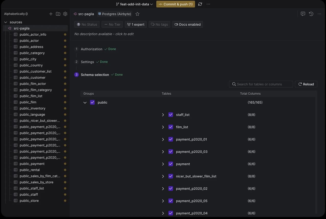
If we take another look at what's ready to be committed, we'll see that the tables we chose are now automatically part of the src-pagila.yml file.

Awesome! Let’s commit these changes and move on to setting up our second source.

Add a custom Python Ingest source

For our second source, we’re going to leverage the country API. While the Pagila database gives us an overview of customer distribution at the country level, it doesn't provide regional-level data. The country API fills this gap, by providing the relationship between countries and regions, among other information.

{
    "af": {
        "name": "Afghanistan",
        "official_name": "Islamic Republic of Afghanistan",
        "topLevelDomain": [
            ".af"
        ],
        "alpha2Code": "AF",
        "alpha3Code": "AFG",
        "cioc": "AFG",
        "numericCode": "004",
        "callingCode": "+93",
        "capital": "Kabul",
        "altSpellings": [
            "AF",
            "Afġānistān"
        ],
        "region": "Asia",
        "subregion": "Southern Asia",
        "population": 2837743,
        ..
    }
}

To get started, you'll need to sign up for a free API key from the country API. Once we have the key, it’s time to store it in Y42. Navigate to the Secrets tab in the Y42 interface and enter your API key there. we will store the API key.

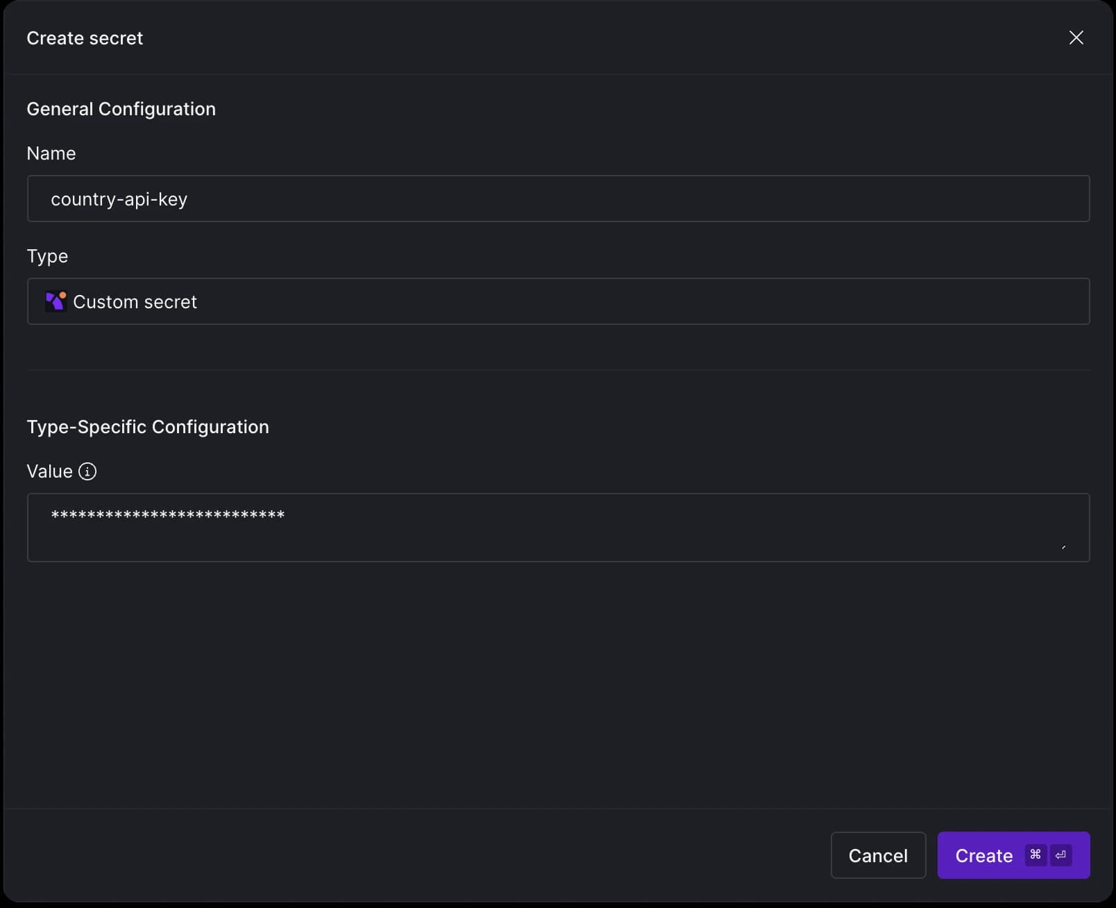
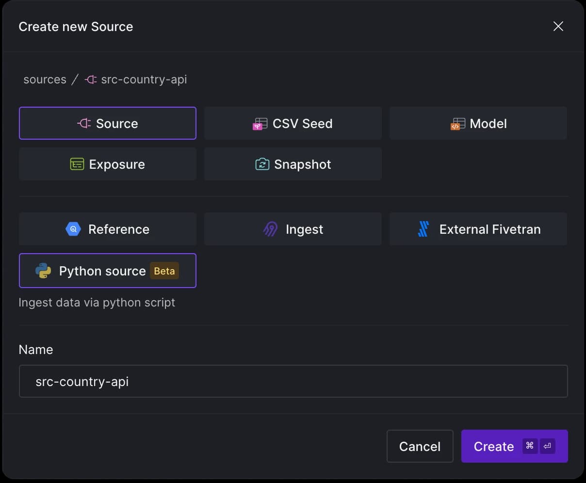
We will use the secret name (country-api-key) when setting up our Python Ingest source. To do this, hit CMD + K in Y42, but this time, choose Python as your Source type.

To extract data from an API using Y42's Python ingest, your code needs to be encapsulated within a function that returns a pandas DataFrame. Y42 simplifies the process by running your code in a Cloud function and then writing the data to your data warehouse. To materialize this function as a source table asset in Y42, we’ll need to use the @data_loader decorator from the y42.v1.decorators module.

import requests
import pandas as pd

from y42.v1.decorators import data_loader

@data_loader
def country_details(context) -> pd.DataFrame:
   base_url = "https://countryapi.io/api/all"
  
   params = {
       "apikey": context.secrets.get('country-api-key')
   }
   response = requests.get(base_url, params=params)

   data = response.json()
   countries_list = [{'name': details['name'], 'region': details['region'], 'subregion': details['subregion']} for key, details in data.items()]
   df = pd.DataFrame(countries_list)
   return df

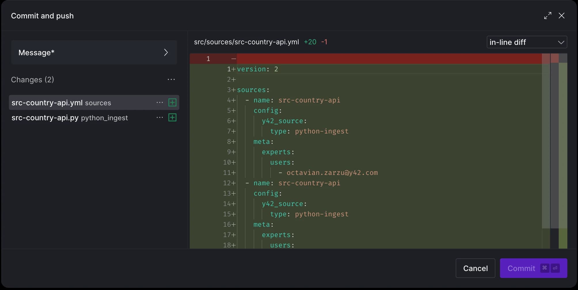
After committing these changes, you'll notice two new files: the Python code you've written and a .yml file containing metadata, similar to what was generated for the Airbyte source

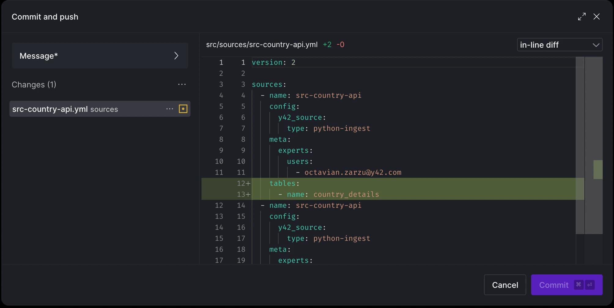
After applying the decorator to the function, the tables section in the .yml file will be automatically updated to reflect the changes:

Model data with dbt

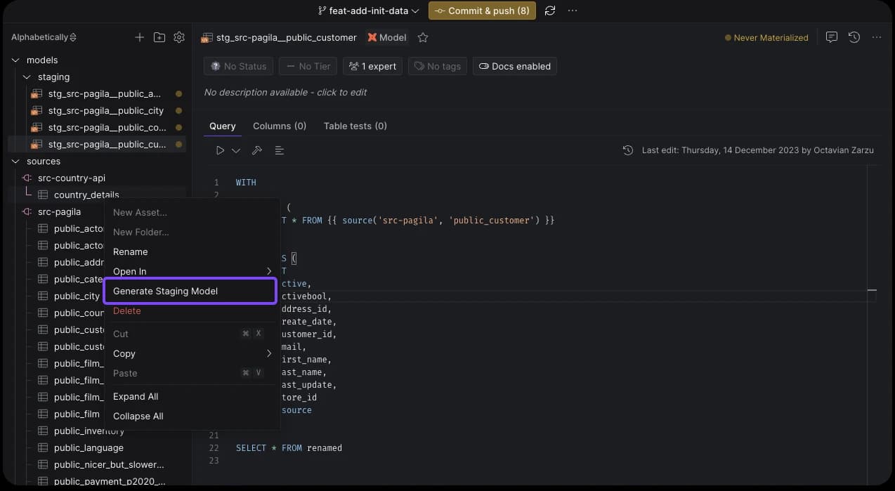
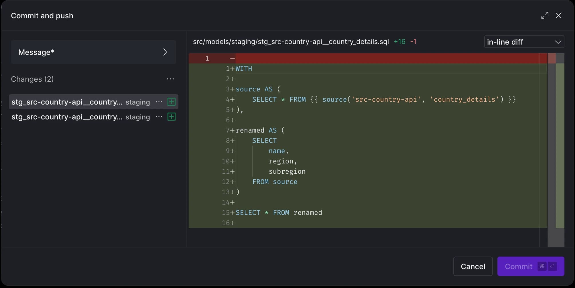
Now, we can build staging tables from all required sources. You can right-click on each source table and select the Generate Staging Model option. This action automatically infers column names and data types from the sources, generating a template .sql and .yml file for each new model.

With just five clicks, we've added five staging table SQL files and their corresponding .yml files!

Committing the 5 generated staging models.

Let’s now create our final model that reports the most popular regions. We will start with the customer asset and navigate our way through the Pagila ER diagram to the country asset, and then join it with the Python API source table.

To begin, hit CMD + K again, and choose model this time:

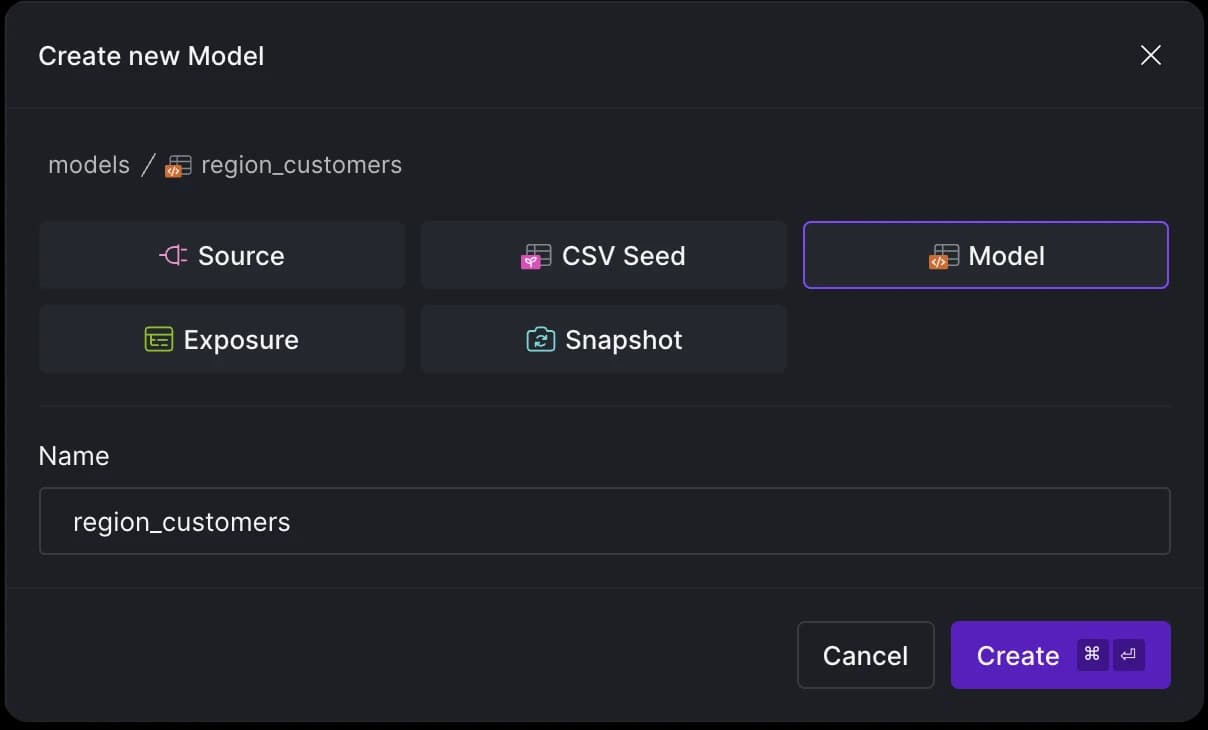
We'll populate our model with the following code:

select
   country_details.region,
   count(cst.customer_id) as customer_count
from {{ ref('stg_src-pagila__public_customer') }} as cst
left join {{ ref('stg_src-pagila__public_address') }} as adr
   on cst.address_id = adr.address_id
left join {{ ref('stg_src-pagila__public_city') }} as city
   on adr.city_id = city.city_id
left join {{ ref('stg_src-pagila__public_country') }} as countryx
   on city.country_id = countryx.country_id
left join {{ ref('stg_src-country-api__country_details') }} as country_details
   on countryx.country = country_details.name
group by country_details.region
having count(cst.customer_id) >= 40
order by count(cst.customer_id) desc

Run pipeline

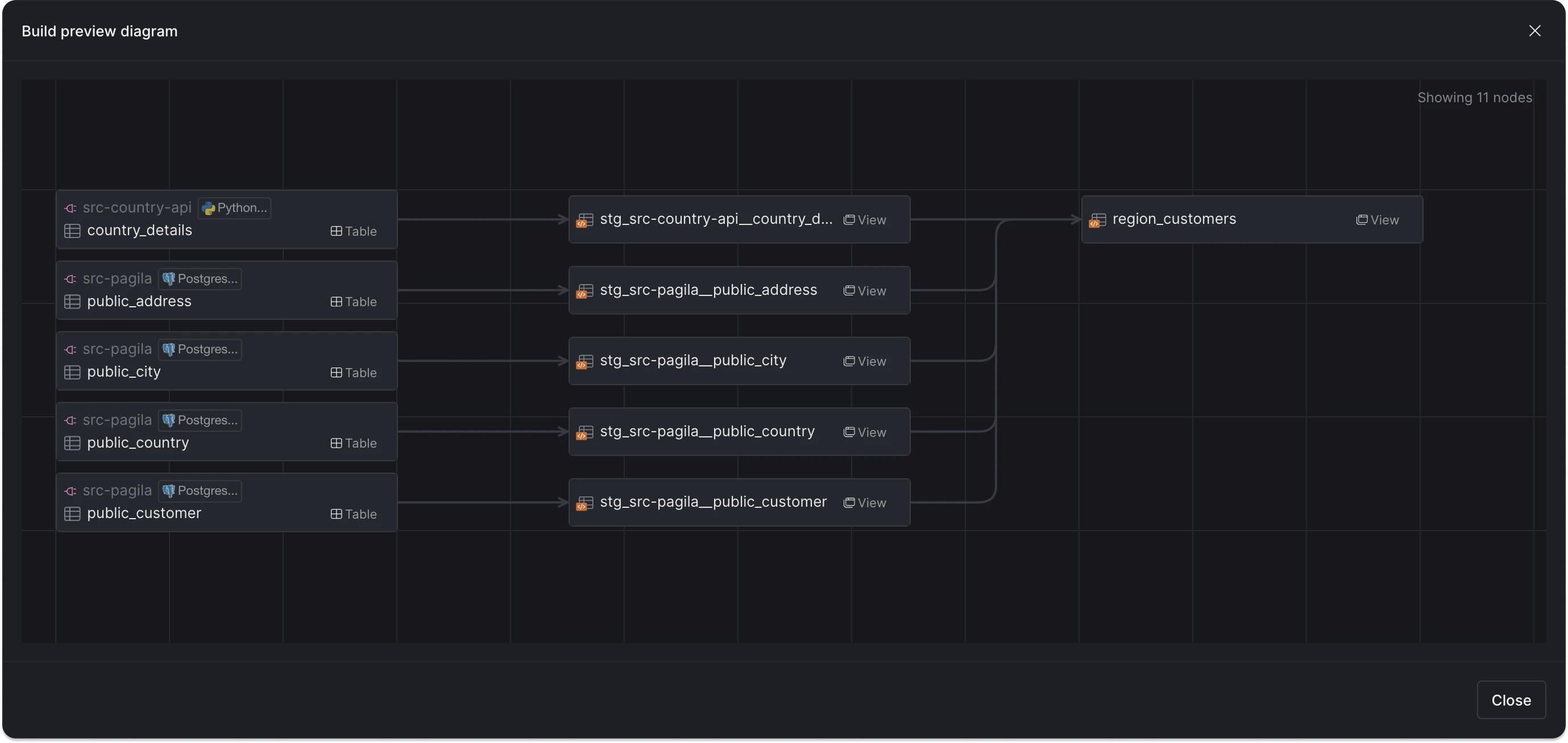
Let's commit our changes and run the pipeline using Y42's DAG selectors:

y42 build -s +region_customers

Using the + in front of the model name allows us to run all upstream dependencies as well. Before running it, we can preview the execution plan to understand what will be processed:

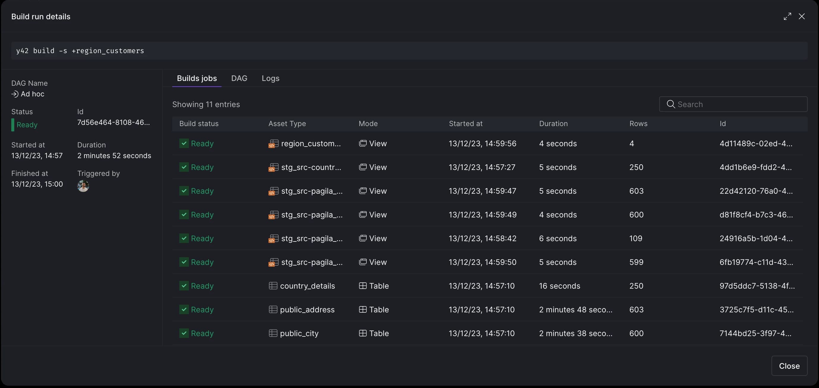
After execution, you can view the run details for each asset:

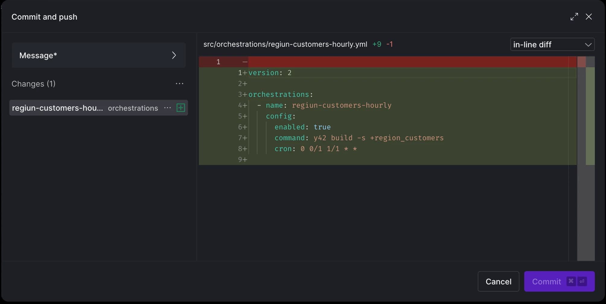
Schedule run

Using Scheduled Builds we can run the pipeline periodically. We can use the same Y42 build command from above, and set the frequency we want the command to run.

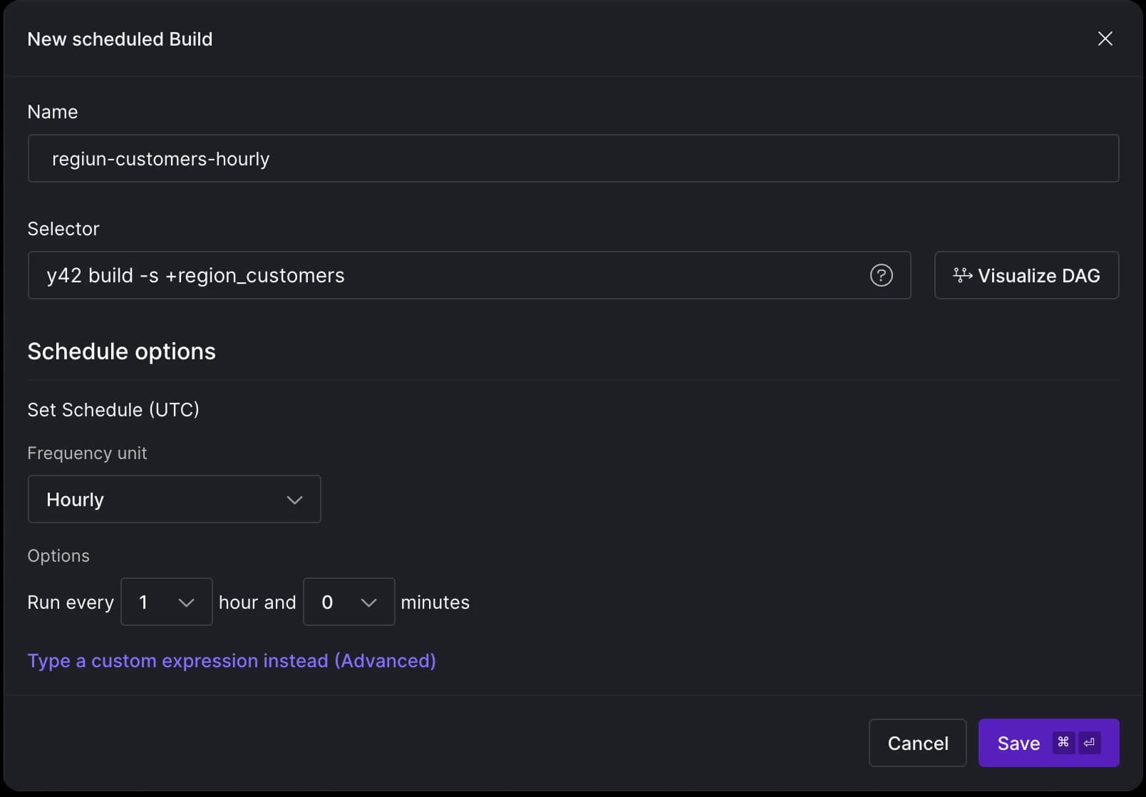
Similar to sources and models, the system tracks scheduled builds and generates a .yml file for it.

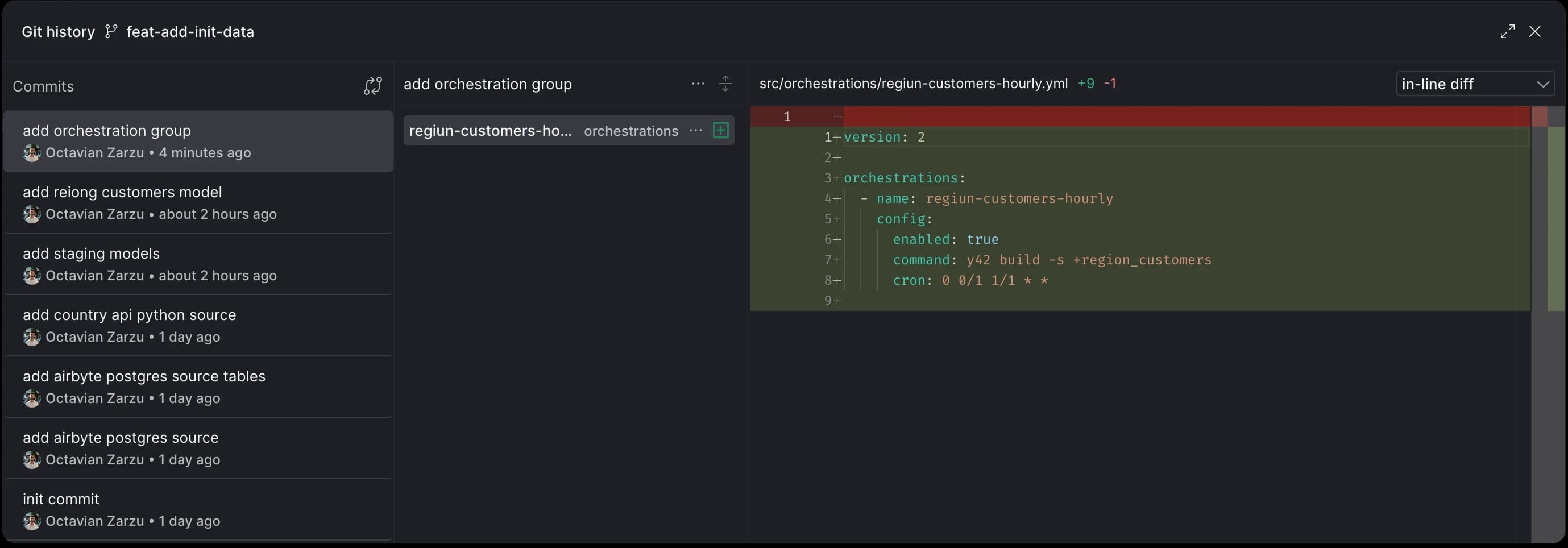
Commit history

With our pipeline set up, we have the option to view the history of all commits using the git commit history option. This allows us to preview commits before merging our branch changes or make any changes by reverting specific commits.

Merge

In our setup we can merge directly to main, however this is highly not recommended. In the next blog entry, we'll explore creating Pull Requests (PRs), running CI checks, reviewing file and asset changes before merging.

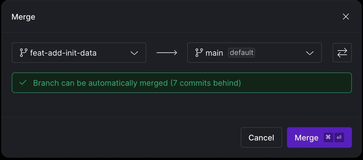
Once we are ready to merge our changes, the Virtual Data Builds mechanism kicks in. The assets we created on the feat-add-init-data branch will also be referenced on the main (production). This means we don't need to rebuild assets, saving compute credits. Similarly, creating a new branch from the main branch for further changes allows us to reuse the same materializations from before. In a nutshell, this lets us work on production data in an isolated environment without impacting the production environment.

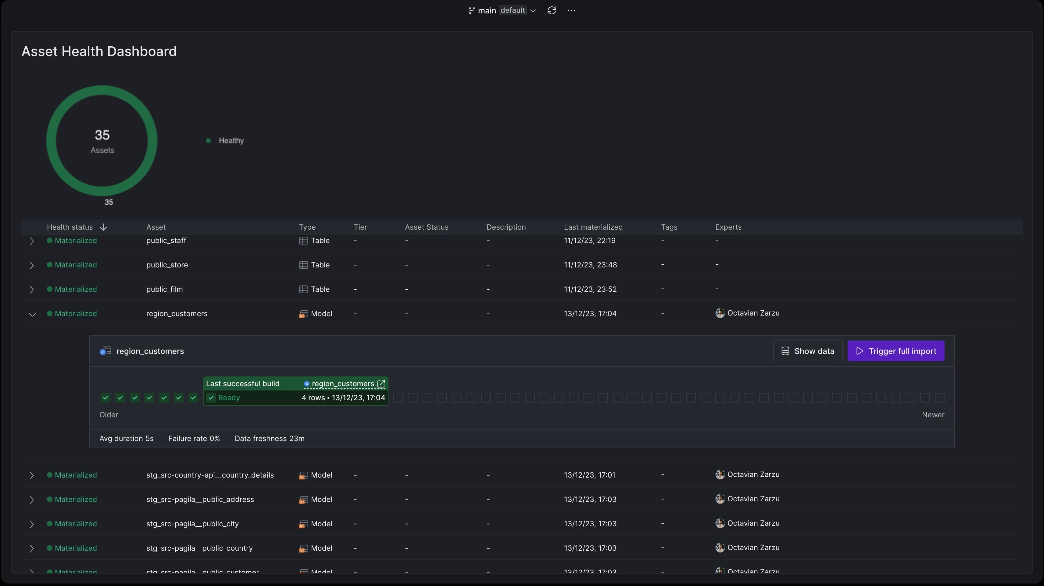
Asset health status

After deployment, the health status of each asset can be continuously monitored using the Asset Health Dashboard:

BI as Code

To close the loop, I'll link to an article discussing BI as Code solutions. There are three options that we'd like to give a shoutout to for embracing the as-code paradigm in the BI layer: Streamlit (Python), Rill (SQL & YAML), Holistics and Evidence (SQL & Markdown).

Conclusion

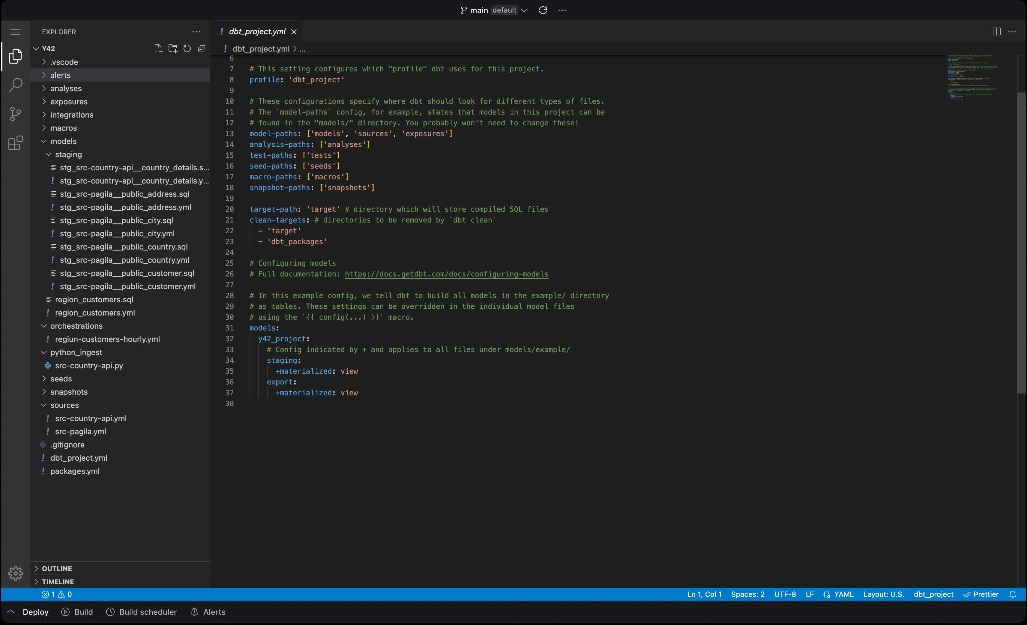
As we've seen, the entire data pipeline creation process can be executed through code in Y42, from defining assets to orchestrating and deploying them. Every UI action for building and deploying pipelines has a corresponding code analog. Each asset is composed of two files: the logic input file and a .yml file containing auto-generated metadata. Alerts, snapshots, seeds, and tests can also be configured via the UI, with corresponding .yml files generated automatically.

For the pipeline we've built above, here's how the in-browser Code Editor view looks now:

Finally, we've explored the merging process within the context of the Virtual Data Builds mechanism, and how assets are reused with zero-compute resources spent on deployment.

In part two, we'll explore how to create Pull Requests in Y42, how the CI bot works, the types of automatic checks performed, and how all these concepts work in an asset-driven world as opposed to one focused on files and tasks. We will also look at some of the new monitoring features and the analytics we can derive from all the standardized metadata we collect and produce when assets are being triggered. Stay tuned!